A shipment arrives with inspection reports showing every checked dimension within tolerance. During assembly, a shaft binds, a cover will not seat, or an internal stack has excessive movement. The immediate reaction is to question machining quality. Sometimes that is justified. Sometimes the supplier has manufactured exactly what the drawings permit, and the permitted combinations cannot deliver the required function.
For global hardware buyers, this distinction affects more than technical discussions. It determines whether the corrective action should be tighter machining control, revised drawings, different assembly rules, or better inspection. Asking for another dimensional report will not solve an incomplete tolerance chain.
This article compares worst-case, root-sum-square, and Monte Carlo analysis using one axial assembly example. All example dimensions and calculated failure rates are educational values from the supplied research, not measured supplier performance. They are identified as [Worked Example] or [Research Simulation]. External references support the methods rather than the invented dimensions.
1. Assembly Tolerance Stack-Up: Why Individually Acceptable Parts Can Fail
Assembly tolerance stack-up refers to the combined effect of permitted dimensional and geometric variation on a functional assembly output, such as clearance, interference, axial movement, or alignment.
A drawing controls inputs. The assembly needs an acceptable output. Those are connected by physical relationships, and inspection of individual inputs does not automatically validate the result. The supplied research describes this result as an assembly response: component variation propagates through the assembly relationship. [Singh and Gulati, Sādhanā]
Consider an ideal cylindrical shaft inside a hole. Diametral clearance equals hole diameter minus shaft diameter. Minimum clearance therefore uses the smallest permitted hole and largest permitted shaft. Subtracting the nominal diameters answers a different question: what happens at the drawing targets?
The same logic applies to an axial stack. If three parts occupy a housing, remaining clearance is housing length minus the three component lengths. A shorter housing and longer internal parts all reduce clearance. Their deviations do not cancel merely because they belong to different components.
This is where supplier discussions often become confused. “All dimensions passed” can describe two different situations. In the first, every applicable drawing requirement was checked and satisfied, but the specification allows combinations that fail function. In the second, only selected sizes were checked, while position, orientation, form, or datum requirements were omitted. The second situation does not establish complete drawing conformity.
A bore can meet its diameter requirement while its axis is unsuitable for the mating arrangement. A spacer can meet its measured length while the surfaces controlling contact introduce an additional assembly effect. Buyers should therefore ask what was measured, how the part was located, and which drawing requirements the report actually covers.
The opportunity is to correct the functional specification before paying for blanket precision. A procurement team that identifies the controlling relationship can focus inspection and machining effort on features that affect assembly. Tightening unrelated dimensions increases cost without necessarily increasing reliability.
There is also a practical ownership question. Who defines the acceptable assembled clearance? Who approves the datum scheme? Who validates operation after finishing and installation? If these responsibilities remain implicit, a supplier may reasonably optimize for the individual drawing while the buyer expects an undocumented assembly outcome.
Define the functional limits before debating whether a tolerance is “tight enough.” State whether parts must interchange freely, whether adjustment is permitted, and which operating condition governs acceptance. A successful trial assembly of selected samples does not establish that every permitted combination will work.
Action recommendation: Add the assembly output, its acceptance limits, and its controlling features to the technical review before releasing component drawings for quotation.
2. Worst-Case Analysis: Testing Whether the Drawing Guarantees Interchangeability
Worst-case tolerance analysis refers to calculating the most unfavorable assembly outputs permitted by the specified input limits and the assembly model.
For a linear chain, each dimension has a signed contribution. With symmetric tolerances, the output tolerance half-width is the sum of each input half-width multiplied by the absolute value of its contribution coefficient. This evaluates permitted extremes, rather than predicting how frequently they occur. [Singh and Gulati, Sādhanā]
Use a housing containing three rigid components, with all dimensions in millimeters:
| Feature | Nominal dimension | Tolerance | Permitted range |
|---|---|---|---|
| Housing length H | 50.100 | ±0.040 | 50.060–50.140 |
| Component length L1 | 20.000 | ±0.030 | 19.970–20.030 |
| Component length L2 | 15.000 | ±0.020 | 14.980–15.020 |
| Component length L3 | 15.000 | ±0.020 | 14.980–15.020 |
The functional requirement is an axial clearance between 0.040 and 0.160 mm. Nominal clearance is 0.100 mm. These dimensions and limits are constructed teaching inputs. [Worked Example]
The assembly equation is:
G = H − L1 − L2 − L3
Minimum clearance occurs with the shortest housing and longest internal components:
Gmin = 50.060 − 20.030 − 15.020 − 15.020 = −0.010 mm
Maximum clearance uses the opposite combination:
Gmax = 50.140 − 19.970 − 14.980 − 14.980 = 0.210 mm
Thus, permitted clearance extends from −0.010 to 0.210 mm, exceeding both functional boundaries. Every contributing dimension can remain acceptable while the assembled result fails. Negative clearance here means axial dimensional overlap in the rigid model, not a shaft-hole interference fit. [Worked Example]
The total tolerance half-width is 0.110 mm, whereas the functional requirement permits only 0.060 mm around the nominal clearance. Merely shifting nominal clearance cannot fit this entire output interval inside the functional window; the permitted variation must also change. [Worked Example]
Possible responses include reallocating tolerances, removing unnecessary interfaces, changing the locating arrangement, or permitting a controlled adjustment. Each option changes a different part of the problem. Tighter machining narrows variation. A shorter chain removes contributors. Adjustment changes how the final output is established.
Worst-case analysis is useful when any accepted replacement component must work with any other accepted component. It does not require assumptions about normal distributions or process centering. However, its guarantee extends only to the model and limits included. An axial calculation that ignores relevant distortion, geometry, or operating effects cannot establish complete functional reliability.
Its conservatism can also create an opportunity. A failed boundary check does not automatically justify tightening every feature. It identifies where the design requires a decision: guarantee interchangeability, introduce adjustment, or approve a defined statistical risk. Procurement should document that decision rather than leave assembly operators to manage it informally.
Action recommendation: Require a reproducible worst-case calculation and resolve any functional boundary violation before accepting a claim of unrestricted interchangeability.
3. RSS Analysis: Predicting Variation Without Confusing Tolerances and Statistics
Root-sum-square analysis refers to combining input variances through an assembly relationship to estimate output variation, including covariance where applicable.
For an independent linear chain, output standard deviation is the square root of the sum of squared input standard deviations, weighted by the dimension coefficients. NIST describes RSS as combining standard deviations and including covariances where appropriate. Its document addresses measurement uncertainty; the propagation mathematics is applicable here, while manufacturing variation remains a separate concept. [NIST Technical Note 1297]
The common shortcut is to insert drawing tolerances directly into that calculation. A tolerance defines acceptance limits. A standard deviation describes observed process spread. Neither automatically determines the other.
For demonstration, assume the four example processes are independent, normally distributed, centered on nominal dimensions, and have tolerance half-widths equal to three standard deviations. These are hypothetical modeling assumptions, not conclusions drawn from a supplier’s rapport d'inspection. [Worked Example]
The assumed standard deviations are 0.013333 mm for H, 0.010000 mm for L1, and 0.006667 mm for each remaining component. The resulting clearance standard deviation is approximately 0.0191485 mm. [Worked Example]
Three standard deviations around the 0.100 mm mean produce an interval of approximately 0.042554–0.157446 mm. This interval fits within the functional limits, even though the worst-case boundaries do not. The analyses answer different questions and therefore do not contradict each other. [Worked Example]
Under the stated normal model, the functional boundaries lie approximately 3.1334 standard deviations from the mean. The calculated probability outside those boundaries is approximately 0.1728%, or 1,728 parts per million. That is a conditional prediction, not a guarantee or an observed production rejection rate. [Worked Example]
Failure also needs a precise definition. This calculation counts insufficient clearance and excessive clearance. It does not say that every failed assembly has physical interference. A component can assemble successfully yet violate the intended axial movement requirement.
Another limitation concerns screening. An untruncated normal distribution includes dimensions outside drawing limits. Consequently, this calculation describes random assembly from the modeled unscreened processes. If production accepts only inspected conforming parts, the input distributions and resulting failure probability need to reflect that selection.
Correlation changes the calculation as well. When two dimensions rise together, their effect depends on the chain signs. Positive correlation increases the variance of their sum but reduces the variance of their difference. Shared machining, locating, or batch conditions should therefore be investigated rather than assumed harmless or automatically harmful. [NIST Technical Note 1297]
RSS offers a practical advantage for stable linear assemblies: it can show which process contributes most to output variation. That helps buyers direct improvement requests toward measurable causes. It also makes the cost of centering visible. Reducing spread will not fully correct a mean that has moved toward a functional boundary.
Action recommendation: Accept an RSS-based yield claim only when the supplier identifies measured means, standard deviations, dependence assumptions, screening rules, and the basis for the probability calculation.
4. Monte Carlo Analysis: Exploring Distribution, Screening, and Process Drift
Monte Carlo tolerance analysis refers to repeatedly sampling modeled component dimensions and calculating virtual assembly outputs to estimate their distribution and functional failure probability.
Its value is flexibility. It can represent asymmetric or truncated distributions, selection rules, and relationships that are difficult to evaluate analytically. JCGM 101 describes propagation of input probability distributions through a model and requires appropriate joint sampling when inputs are dependent. Like the NIST reference, it is a metrology document whose mathematical framework must be applied carefully to manufacturing. [JCGM 101:2008]
The supplied research reports one million virtual assemblies for each of three input models using the same drawing limits. The following results are reported simulations, not measured CNC production outcomes. [Research Simulation]
| Input model | All modeled parts within tolerance? | Functional failures | Estimated failure rate |
|---|---|---|---|
| Independent centered normal, without truncation | No | 1,710 | 0.1710% |
| Same normal model, truncated at individual limits | Yes | 1,146 | 0.1146% |
| Independent uniform distributions within limits | Yes | 67,228 | 6.7228% |
The first model agrees closely with the RSS prediction. The second demonstrates the central procurement issue: screening every individual dimension can still leave assembly failures. The third shows that identical tolerance limits can produce substantially different risks when the dimensions occupy those limits differently. [Research Simulation]
Uniform inputs spread probability across the full permitted interval. The centered normal models concentrate more values near the targets. Neither distribution should be selected because it produces a preferred result. The supplier needs evidence that the chosen model represents the delivered population, including any inspection or sorting.
Process drift introduces another risk. In the teaching case, shifting the housing mean from 50.100 to 50.080 mm while keeping other means and standard deviations unchanged moves mean clearance to 0.080 mm. The modeled failure probability rises to approximately 1.8372% under the untruncated normal assumptions. [Worked Example]
A simulation based on historical centered data will miss that change unless the input model is updated. NIST’s capability guidance compares a stable, in-control process with specification limits; familiar capability indices also depend on distribution assumptions. A selected sample histogram is insufficient evidence that future production will behave the same way. [NIST/SEMATECH Engineering Statistics Handbook]
Simulation count also matters. Repeated runs have sampling uncertainty, particularly in the failure tail. The supplied normal-model result has a reported approximate 95% failure-rate interval of 0.1629–0.1791%. More runs narrow simulation sampling error, but cannot correct an incorrect distribution, missing correlation, or incomplete assembly model. [Research Simulation]
Action recommendation: Request the input-data basis, selection logic, model version, run count, dependence treatment, and failure-rate interval before using simulation results to approve production.
5. Procurement Validation: Turning Tolerance Analysis into Supplier Evidence
Procurement validation refers to checking that drawing requirements, production data, analysis assumptions, and physical assembly results collectively support the required function.
The practical objective is traceability. A buyer should be able to follow the argument from the current drawing through measured inputs to a predicted output and an actual assembly check. A polished simulation image or a single capability number leaves too much of that argument unexplained.
For the teaching assembly, an effective review begins with the 0.040–0.160 mm functional requirement and the four contributing dimensions. Those values define what the model must explain. Without an agreed functional window, a reported failure percentage has no stable meaning. [Worked Example]
Request evidence in a sequence that exposes errors early:
| Evidence | What the buyer should verify |
|---|---|
| Functional requirement | Limits, operating conditions, failure definition, and approved risk |
| Current drawing and chain | Revisions, units, contribution signs, interfaces, and applicable geometry |
| Worst-case calculation | Permitted extremes compared with functional boundaries |
| Production measurements | Raw values with dates, batches, processes, and measurement methods |
| Statistical model | Means, spreads, distributions, dependencies, and selection rules |
| Physical validation | Predicted outputs compared with measured mating assemblies |
| Change control | Conditions requiring reassessment of the approved analysis |
This is a proposed purchasing checklist, not a claim that one standard mandates this exact document package.
Raw data matters because a summary can conceal mixed populations. Measurements from different machines, setups, or batches may create patterns that disappear in an overall average. Ask whether the model represents parts shipped together, randomly mixed inventory, or deliberately matched sets.
Measurement validity matters for the same reason. Calibration status, measurement uncertainty, locating methods, and repeatability affect how confidently observed spread can be interpreted. Buyers should avoid treating every fluctuation in measured data as manufacturing variation without examining the measurement system.
Physical validation closes the model. Pair identifiable components, enter their measured dimensions into the chain, and compare predicted clearance with the assembled result. If prediction and observation disagree, investigate omitted geometry, contact rules, deformation, or measurement differences before presenting the model as validated.
There are several legitimate commercial responses to a failed tolerance analysis. The design can change. Critical tolerances can narrow. Assembly can include adjustment. Components can be selectively matched. Each option has consequences for production cost, replacement parts, traceability, and service. Selective assembly may work for initial production while making unrestricted field replacement difficult.
An RFQ should therefore request a reproducible tolerance-chain report for specified functional outputs. If statistical approval is proposed, require representative data, assumptions, screening rules, predicted failure rates, and validation evidence. Assign approval responsibility to the buyer’s engineering function and identify which process changes require renewed review.
This approach creates negotiating clarity. Instead of demanding “better quality” without a defined target, the buyer can ask for a specific functional outcome and evidence that the chosen controls deliver it. Supplier effort then addresses the real source of assembly risk.
Action recommendation: Make assembly-function evidence a technical acceptance item and connect its approval to drawing revisions, production conditions, and replacement-part requirements.
Foire aux questions
R : Yes. Individual limits may allow combinations outside the assembly’s functional limits. Alternatively, the inspection may cover only selected dimensions rather than every applicable requirement. Establish which situation occurred before assigning corrective action.
R : No. It establishes permitted boundaries within the model. Predicting frequency requires information about process distributions, centering, dependencies, and assembly or screening rules.
R : No. That relationship requires supporting process evidence. A tolerance is an acceptance requirement; standard deviation describes spread. Treating them as interchangeable can produce misleading yield estimates.
R : No. Accuracy depends on the inputs and model. RSS can be efficient for a linear chain with justified statistical assumptions. Monte Carlo is useful when distributions, selection, or geometry require more flexible propagation.
R : No. Component capability compares one process output with its own limits. Assembly reliability depends on the combined functional output. Good component capability supports the analysis but cannot replace it.
R : Request the functional limits, current drawings, actual mating-part measurements, and the assembly equation. Use these to distinguish nonconforming manufacture, incomplete inspection, and insufficient design limits before deciding whether tighter machining is needed.